Related Work

Traffic signal recognition is a technology by which a vehicle is able to recognize different traffic signs and it is part of features collectively called ADAS (Advanced Driver Assistance Systems) [1]. It uses image processing techniques to detect traffic signs and the detection method can be generally divided into color based, shape based and learning base methods.

The first TSR systems which recognized speed limits were developed in cooperation by Mobileye and Continental AG in 2008. But, these systems only detect the round speed limit signs found all across Europe.

Since 2012, Volvo is working on a technology called Road Sign Information but they are not able to recognize city limit signs in many European countries because they are too similar to the direction signs.

Vehicle detection research varies from using active sensors to using passive sensors. Active range finding sensors have had success, but are quite expensive and tend to be single-purpose. They can track cars ahead, but cannot be used to detect lanes, road curve, road type, signs, and other obstacles [2].

Modern traffic sign recognition systems are being developed using convolutional neural networks, mainly driven by the requirements of autonomous vehicles and self-driving cars. In these scenarios, the detection system needs to identify a variety of traffic signs and not just speed limits. This is where the Vienna Convention on Road Signs and Signals comes to help. A convolutional neural network can be trained to take in these predefined traffic signs and 'learn' using Deep Learning techniques.

There are diverse algorithms for traffic sign recognition. Common ones are those based on the shape of the sign board. Typical sign board shapes like hexagons, circles, and rectangles define different types of signs, which can be used for classification. Other major algorithms for character recognition includes Haar-like features, Freeman Chain code, AdaBoost detection and deep learning neural networks methods. Haar-like features can be used to create cascaded classifiers which can then help detect the sign board characters [3].

Our work expands into the area of traffic “STOP” sign using a Bag-of-Words approach and the images are convolved using a difference of Gaussian filter bank. The responses from the filter bank are applied to a precomputed set of principle components. The idea of the difference of Gaussian filters comes from how the brain interprets line segments [4]. Responses from the visual cortex have been recorded as similar filters. The idea is that these primitive filters combine to represent all that we see and can interpret.

Our object detection procedure classifies images based on the value of simple features. There are many motivations for using features rather than the pixels directly. The most common reason is that features can act to encode ad-hoc domain knowledge that is difficult to learn using a finite quantity of training data [5]. For this system, there is also a second critical motivation for features: the feature based system operates much faster than a pixel-based system.

Method

This project uses the data available on the LISA Traffic Sign Dataset [6]. Although there are more than 6000 frames present in the aforementioned dataset with more than 47 sign types, we chose 5 different types of signs, namely – ‘STOP’, ‘ADDED LANE’, ‘PEDESTRIAN CROSSING’, ‘SIGNAL AHEAD’ and ‘KEEP RIGHT’ for simplicity sake. We chose all the images for each of the 5 types of street signs, making a total of 2,024 images as the input data.

We split this data into 50 images to test the model and the remaining images for training the model. Each sign type is assigned a categorical value, and they are as follows – ‘Keep Right’ – 1, ‘Signal Ahead’ – 2, ‘Stop Sign’ – 3, ‘Pedestrian Crossing’ - 4, ‘Added Lane’ – 5. We use the training data to make the model learn about the data and extract the features from the data. The testing data is used to check if our model is indeed working the way we intend it to work.

Firstly, not all the images in the dataset were annotated with labels, and they were not segregated by sign type into their own folders. So our first task was to sift through all of the images present on the dataset, and pick out the ones which belonged to the 5 classes that were picked. Once the required files were obtained, we then had to segregate them into their own folders depending on which sign type it was. Then each file was assigned the labels mentioned above.

Once we have all the data present in the requisite format, we then need to use 4 types of filters on the image with 5 varying parameters (scale) in each of them. Since color images have 3 channels, we will have a total of 3F filter responses per pixel if the Filter Bank is of size F. We also have to transform the image from the RGB color space to the Lab color space. The 4 filters which are also shown in Figure 1 are as follows:

• Gaussian – this type of filter is used to obtain a filtered image using a 2-D low-pass Gaussian smoothing kernel, it is used for blurring the image to remove the noise and yet preserves high frequency components
• Laplacian of Gaussian (LoG) – this filter is obtained by calculating the Laplacian of a Gaussian filter, it is used for edge detection as it highlights regions of rapid intensity change
• Oriented Gaussian in X Direction – this filter is used to detect any horizontal edges or lines in the images
• Oriented Gaussian in Y Direction – this filter is used to detect any vertical edges or lines in the images e

Figure 1 – Filters used

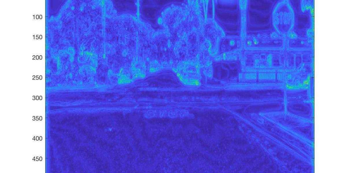
The 5 different parameters used for scaling the filter are : [1 2 4 8 *8]. An example of an image taken (Shown in Figure 2) containing a ‘STOP’ sign upon filtering is shown in Figure 3.

Figure 2 – Original image

Figure 3 – Montage of all filters applied to the image

Once we have the filtered images, we have to pick a number of pixels (α) from the image, and this number was chosen to be 100 after multiple rounds of trial and error.

With these random pixels, we calculate the dictionary [7] for each image. We store the dictionaries of all the “  .png” in a single “dictionary.mat” file. This project uses a Bag of Words (BoW) Approach. It combines this with Spatial Pyramid Matching and Feature Encoding [8]. This represents an image as a visual-word vector. Thereafter, the comparison between images is realized in the visual-word vector space. Finally, we will build a sign detector based on the visual bag-of-words approach to classify a sign-board image into 5 distinct classes.

We calculate the dictionary for each image by performing a k-means clustering of the filter responses. And we pick the k value to be 150 clusters after performing several experiments and found this value to be the optimal one. Perhaps giving a larger number of clusters could in theory give us better performance and accuracy, but due to time-constraints and for practical purposes, the value was kept as 150.

Now that we have the “dictionary.mat” file, we need to create the visual words for all the images. We use the standard Euclidian Distance (pdist2) to assign the closest visual word of the filter responses to the respective pixel in the image. Upon running the batchToVisualWords, we get a wordMap generated for each image in the dataset.

One such wordMap for “STOP” sign image is shown below in Figure 4.

Figure 4 – Example of a wordMap

Next, we must generate a histogram for each image by giving the wordMap and the number of “bins” as Dictionary Size, which is also the same as the number of clusters in our k-means classifier i.e. 150.

Our approach currently discards information about the spatial structure of the image and this information is often valuable, thus we need to perform Spatial Pyramid Matching [9][10]. In this approach, we divide the image into a small number of cells, concatenate the histograms of each of these cells to the histogram of the original image, with a pre-determined weight for each layer. In our Spatial Pyramid, we have 2 layers. Level 2 corresponds to the image being divided into 16 portions, histogram is calculated from these portions, and in Level 1, the image is divided into 4 parts, and a histogram is calculated from these 4 parts. Then L1 normalize the vector.

Our next step would be to find the histogram intersection similarity between each image in the testing set is compared with all the histograms in the training set, and we can do this in a parallel manner using the MATLAB function bsxfun. This is called the nearest neighbor approach which was used by James Hyatt et. al [11].

We then save the training data, along with the filterBank, dictionary as well as the training labels in a MATLAB file called “vision.mat”. We then take the histogram of the test data and compare it to the histogram of the training set and take the one which is the largest value, because we are comparing a degree of “similarity”. Then the label of that image in the training set is assigned to this image in the test set. Similarly, this process is repeated for all 250 samples present in the test dataset. We then build the confusion matrix, comparing the predicted labels generated by our model with the actual labels of each of these images. The evaluateRecognitionSystem.m is the code that generates this confusion matrix, which gives us our class by class as well as final accuracy.

Results

The results for this image detector were very positive. First, we created our traintest.mat with images from our dataset. We used 5 sets of image types: Keep Right, Pedestrian Crossing, Signal Ahead, Added Lanes and Stop Signs. For Keep Right we used 140 images with 90 for training. For Pedestrian Crossing we used 725 images with 675 for training. For Signal Ahead we used 317 images with 263 for training. For Added Lanes we used 178 images with 128 for training. For Stop Signs we used 664 images with 614 for training. For all of our categories we used 50 testing images for each.

The training test was used to extract features of our images, while the test images are used to test our programs accuracy. For every image in our training set, a histogram of visual words is extracted from our dictionary map using the code present in getImageFeatures.m. Below in Figure 4 there is an example of a histogram from a particular image.  The histograms of the images in the testing data set are compared to the histograms of all the training set images.

The testing set is used to test the accuracy of our program and results in a confusion matrix to show the accuracy per image type. The confusion matrix that was generated at the end gave us very high image detection. For Keep Right, 47 images were guessed correctly while 3 images were guessed incorrectly (refer to the first row of figure 5 below). For Signal Ahead, 45 images were guessed correctly while 5 images were guessed incorrectly (refer to the second row of figure 5 below). For Stop Signs 49 images were guess correctly while 1 image was guessed incorrectly (refer to the third row of figure 5 below). For Pedestrian Crossing, all images were guessed correctly (refer to the fourth row of figure 5 below). For Added Lane, 37 images were guessed correctly while 13 images were guessed incorrectly (refer to the fifth row of figure 5 below).

Overall the accuracy was 91.2 percent, refer to Figure 5 below for the confusion matrix. The categories that were guessed the most correct had the highest data set size for training images. For example, Pedestrian Crossing had the highest accuracy rate of 100 percent. This may be due to it having the highest data set for training. On the other hand, Added Lane had the lowest accuracy of 74 percent. This may be due to it having the lowest data set size for training.

                                             Figure 4 – Example of a histogram

                                                  Figure 5 – The final confusion matrix

Conclusion and Future Work

As this is a safety critical system, the accuracy of this when used in the real world must be as close to 100% as possible to prevent human loss of life or property. To improve our current accuracy of 91.2% to a 99.9% will be challenging, but given below are a few of the methods to increase the accuracy of classification in future endeavors of this project.

A way to increase accuracy would be to increase our data set size drastically. In this case we are using 2024 images totally, but this a very small number when it comes to a real world application. If this exercise is performed on a large scale (10s of thousands or 100s of thousands images) than we could increase the accuracy to almost 100 percent.

Another idea would be to bump up all the parameters, such as α even more, however it’s a trade-off between accuracy and time. As the parameters and data set sizes increase, the time for the code to run also increases. This is a direct correlation and is something to take into heavy consideration. In this approach we used k-means with spatial pyramid mapping. It may be possible that if we took the convolutional neural network approach that this could also increase the accuracy of our results. We could include other traffic signals also which would resonate to more real world scenarios.

Another approach which can be taken into consideration in future is the use of other types of filters like Gabon filters or Kalman filter. We believe this will somewhat result into increased accuracy and better recognition of traffic signals due to better filter responses extraction. We can also try and see if increasing the number and value of the scales used along with filters has an impact on the final accuracy.

Even though preliminary results are promising, in future we can directly feed the video from a moving vehicle to our Gaussian mixture model. This will increase the run time of the system and train it to work better with more accuracy in real world scenario.